The Sciences: Astronomy & Astrophysics:

 

Is a Single, Finite, Open Universe

Ruled Out by Planck’s Satellite Data?

By Dr. Julio A. Gonzalo.

Escuela Politécnica Superior, Universidad San Pablo CEU, Montepríncipe

Madrid, Spain

and Departamento de Física de Materiales, Universidad Autónoma de Madrid

Madrid, Spain

and

Dr. Manuel Alfonseca

Escuela Politécnica Superior, Universidad Autónoma de Madrid

Madrid, Spain

 

Abstract

Since 1998, when the unexpectedly accelerated expansion of the universe was first reported, it has become customary to describe the universe using the LCDM model. The implicit critical assumption of a non-zero cosmological constant and a null space curvature is shown here to be open to question. The availability of exact analytical solutions for Einstein cosmological equation in the L-Cold Dark Matter and the K-Open Friedman-Lemaitre models makes it easy to quantitatively compare different models of the universe regarding the existence and proportion of dark matter and energy, the CMB anisotropies, the maximum observed redshifts, the average cosmic density and other cosmic quantities. The fact that both models, as well as intermediate ones, fit many of the experimental data reasonably well, while they are still prone to criticism in different places, can be taken as proof that further investigation is needed.

Keywords: cosmological parameters; cosmology: theory; dark matter; dark energy; large-scale structure of universe

1. PRELIMINARY CONSIDERATIONS: A HISTORICAL REVIEW

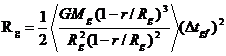
For about a century, quantitative discussions of astrophysical cosmology have taken as the starting point Einstein’s cosmological equations, that can be put into condensed form in the single equation:

,                                                               (1)

Hereis the time derivative of the radius of the observable universe R,  is the finite mass of the universe, including the observable universe and that part of the plasma universe beyond the sphere of the CMB which is not directly observable (with  its average density), G = 6.67 ´ 10^-11 IS units is Newton’s gravitational constant, k the space-time curvature, c = 3 ´ 10⁸ m/s the speed of light, and L (m^-2) the cosmological constant.

We assume that equation (1) describes correctly the cosmic evolution at least as a first approximation. General compact solutions of equation (1) are used below to investigate what values of k and L are compatible with the available observational evidence, especially with reasonable values of Hubble’s parameter (Livio & Riess 2013)  and with the age of the universe,  t₀.

It is well known that in the early 1950’s there were two competing models, based upon very different interpretations of equation (1), to describe the apparently isotropically expanding universe: the Big-Bang model (first proposed by G. Lemaitre and later developed by G. Gamow, R.A. Alpher and R. Herman), and the Steady State model (developed by T. Gold, H. Bondi and F. Hoyle). The second model postulated a continuous creation of matter out of nothing to keep (artificially) constant the cosmic density during the expansion. The discovery of the 3 K cosmic background radiation by A. Penzias and R. Wilson in 1966 made the Steady State model untenable, but its assumption of spontaneous creation of matter or energy through volume increase at constant density resurfaced some years later in the inflationary model.

Theories involving multiverses (Rees 2000), an infinity of universes, each with a different set of universal constants, became fashionable in the last decades of the 20^th century. According to most of these theories, our universe is completely disconnected from all other hypothetic universes and there is no possibility of exchanging information with them. Anyway, we are primarily interested in our own universe, characterized by the fixed set of universal constants that have been painstakingly determined with ever increasing precision by actual physical observations.

Theoretical cosmologists point out sometimes that it is difficult to chose between an infinite universe and an enormously large one. This may be true in the abstract, but it must be noted that an actually infinite universe leads to problems with equation (1). If M is actually infinite, the second and the third terms (involving a finite k and a finite L) become totally irrelevant.

It is true that k£0 in equation (1) implies that the geometry of the universe is potentially infinite, but to make it actually infinite, one has to add an additional postulate, namely the so-called cosmological principle, which asserts that the universe is indefinitely homogeneous and isotropic at sufficiently large scales. However, Olbers gravitational paradox (Jaki 2000) cannot be explained away convincingly except for a universe with a finite mass. Therefore a flexible position with respect to the extrapolation of the known universe beyond our horizon is at least epistemologically reasonable, especially when that extrapolation leads to infinity. In fact, Einstein, Friedman, Lemaitre, Eddington and others (Einstein 1952) always assumed a finite mass for the universe, for both the open, flat and closed cases. Astronomers estimate that the visible universe contains about 10¹¹ galaxies, each with about 10¹¹ stars with an average mass of the order of the Sun’s mass (10³⁰ kg), which results in a total mass  kg, enormous but finite.

When Einstein boldly made the original attempt to use his general theory of  relativity to describe the cosmos as a whole, he evidently had in mind the three particular physical cases where he had applied successfully his general theory of relativity (Gonzalo, 2012): the bending of light in the Sun gravitational field, the advance in the perihelion of Mercury, and the gravitational redshift of light emitted by very massive objects. In those three cases he had taken k > 0, and it is likely that he originally expected that k > 0 in equation (1) would describe the whole cosmos. For this reason he introduced the third term with L, in order to achieve a static universe. Much later, in 1947, he said in a letter to Lemaitre (Gonzalo 2012, p. 61):

Since I introduced this term I had always a bad conscience. But at the time I could see no other possibility to deal with the fact of the existence of a finite mean density of matter. I found it very ugly indeed that the field law of gravitation should be composed of two logically independent terms which are connected by addition. About the justification of such feelings concerning logical simplicity it is difficult to argue. I cannot help to feel it strongly and I am unable to believe that such an ugly thing (two terms connected by addition) should be realized in nature…

On the other hand, it was perfectly reasonable, as Friedmann and Lemaitre did, to take k < 0, in which case the third term (with L > 0) would be unnecessary. In fact, during the expansion, especially in the early phase, when the cosmic background radiation density was very high, the radiation pressure would have overcome by far the gravitational attraction. In other words, a negative k would have an obvious counter gravitational physical meaning, not suspected by Einstein at the time of writing down equation (1).

2. COSMOLOGICAL MODELS AND THEIR VALIDATION

Since 1998, when the unexpectedly accelerated expansion of the universe was first reported, it has become customary to describe the universe using the Lambda Cold Dark Matter (LCDM) model, which assumes k=0 L>0 in Einstein equation (1).

Whether cosmic space-time curvature is closed, flat or open must be decided, of course, on experimental grounds. However, at present this is not always done. (Ade et al, 2013), for instance, present a computation of cosmological parameters to fit the experimental results obtained by Planck satellite. In their paper, they describe the procedure they have used, which can be summarized thus:

1.                  They postulate the LCDM model, i.e. a flat universe (k=0, L> 0) with six free parameters, each of which with a given starting range: w_b [0.005, 0.1], w_c [0.001, 0.99], q_MC [0.005, 0.1], t [0.01, 0.8], n_s [0.9, 1.1] and A_s [1.49E-9, 5.46E-9] (see Table 1 in Ade et al, 2013). The range for the starting values of four of these parameters is quite ample, as it encompasses more than one and up to three orders of magnitude.

2.                  They adjust the values of those six parameters so that their model fits the experimental data. Obviously they start adjusting the values of the two parameters with the smallest allowed range amplitude (the last two) and then tune the other four. With such a number of free handles, the fact that they could find a proper fitting is not so surprising. Table 2 in their paper show the values they have obtained for the six free parameters.

3.                  They next use those adjusted parameter values to compute the values of other cosmological parameters in the LCDM model, such as H₀, t₀, and W_m. Table 2 and 5 in their paper shows three different sets of values, obtained by using the Planck satellite experimental results alone, or combined with other results (lensing data, WMAP low-l polarization, high resolution CMB data and baryon acoustic oscillation surveys). Depending on the data combination used, the best fits and the 68% adjustment intervals obtained are somewhat different. For the three variables mentioned above, the union and the intersection of the 68% intervals found are respectively: H₀ [66.0, 69.4] [67.03, 68.5] km/seg/Mpc; t₀ [13.738, 13.871] [13.769, 13.835] Gyrs; and W_m [0.288, 0.334] [0.298, 0.318]. The best fits used vary with the source, but those frequently given are: H₀ = 67.15, t₀ = 13.798 Gigayears, and W_m = 0.319. Observe that, since the estimated relative density of baryonic (non-dark) matter  is 0.049, the relative density of dark matter is automatically computed as W_dm = W_m-0.049 = 0.268, while the relative density of dark energy is also automatically computed as W_L = 1- W_m = 0.683, to assure that the universe is flat (k=0), the starting point of the whole computation.

4.                  In section 6 of the paper, the curvature of the universe, as deduced from their results, is said to be very small, of the order of W_k = 0.001, and this is given as a proof that the paper has validated the LCDM model.

Has the LCDM model been really validated? Having been chosen as the starting point, it is not surprising that a low value of W_k comes out of the computations. In fact, the authors of the paper are aware of this, for they write (Ade et al, 2013, page 2):

“Figure 1 is based on a full likelihood solution for foreground and other “nuisance” parameters assuming a cosmological model. A change in the cosmology will lead to small changes in the Planck primordial CMB power spectrum because of differences in the foreground solution.”

In computer simulation, the validation of a model, after it has been adjusted to the available experimental data, can be done in two different ways. The first is best, but not always possible, when the second alternative may be used:

a)                 By using the model to make predictions of possible results, different from those used to adjust the model and confirming those predictions with new experimental results. In principle, measurements of W_m(z) in successive intervals (z, z+dz), are possible.

b)                 By comparing the model with other available models and coming to the conclusion that this model fits better the available data. In this case, the best-fitted model is accepted provisionally as the good one, until new experimental data make a proper validation possible.

In the following section we shall offer a comparison of several models (LCDM, KOFL, and a family of mixed models) and will try to signal the current strengths and deficiencies of the first two.

 

 

3. COMPARING DIFFERENT COSMOLOGICAL MODELS

To compare different cosmological models, we have started from reasonable values for the two cosmological parameters H₀ and t₀, and used equation (1) to find comparable results. Of course, we are discarding an infinite M, which would make the equation useless, and adjust its finite value and that of R₀ to obtain the desired values for H₀ and t₀. As the sphere occupied by the cosmic microwave background radiation separates the visible (transparent) universe from the opaque (plasma) universe, not all of the mass (matter and radiation) in the universe is directly observable.

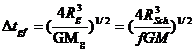
Table 1

Comparison of three different cosmological models: a flat (ΛCDM) universe (top-left) with k=0, an open (KOFL) universe (top-right) with Λ=0 and a mixed universe (bottom) with Λ= Λ₀/2, k=-0.5. In all three, R_1/2=R[W_m=1/2]_.

 

Radius	ΛCDM, H0=67.15, t0=13.798, Λ=1.0764.10-52 m-2, M=2.9595.1052 kg, T0=2.72548 K.					KOFL, k=-1, H0=66.55, t0=13.75, M=4.9527.1051 kg, T0=2.72548 K.
	R (Mly)	t (My)	z	T(K)	Wm	R (Mly)	t (My)	z	T(K)	Wm
R0	14562	13798	0	2.7255	0.319	15067	13750	0	2.7255	0.0491
R1/2	11310	10369	0.2875	3.5091	0.5	777.5	414.3	18.38	52.817	0.5
RSch	4646	3063	2.134	8.5423	0.935	777.5	414.3	18.38	52.817	0.5
RCMBR	13.23	0.47	1099.7	3000	1	13.69	1.205	1099.7	3000	0.983

 

Radius	Mixed, H0=67.15, t0=13.798, Λ=0.5382.10-52 m-2, k=-0.5, M=1.9114.1052 kg, T0=2.72548 K.
	R (Mly)	t (My)	z	T(K)	Wm
R0	15409	13798	0	2.7255	0.1739
R1/2	5429	3923.5	1.84	7.74	0.5
RSch	3000	1758.5	4.14	14	0.660
RCMBR	14	0.92	1099.7	3000	0.9977

 

The values we have used for H₀ and t₀ with the LCDM and the mixed model are those obtained as best-fit in the (Ade et al, 2013) paper. Therefore, as was expected, the value obtained for W_m0 is also the same, which confirms that our procedure is correct. For the Open Friedman–Lemaitre (KOFL) model, however, we have used slightly different values for H₀ and t₀, keeping them in both cases in the 68% interval postulated by (Ade et al, 2013). Notice that, once the two free parameters (M and R₀) have been adjusted to the desired values of  H₀ and t₀, the value of Λ with the LCDM model is automatically derived from equation (1). Notice also that the value adjusted for M is of the same order of magnitude as the estimation for baryonic mass in section 1, and that R_1/2 and R_Sch are the same for the KOFL model and different for the LCDM and the mixed model.

The difference between the three models is obvious: in the KOFL model, W_m0 = 0.0491, which means that all the mass in the universe is baryonic, so, properly speaking, there is neither dark matter nor dark energy (Λ=0 in this model). In fact, the exact value of barionic matter could be increased and a certain amount of non-luminous dark matter could be introduced, simply by adjusting slightly the values of the two parameters, H₀ and t₀. In the LCDM model, however, W_m0 = 0.319, which (assuming that W_b = 0.0491) corresponds to a dark matter relative density equal to 0.268, as stated in the Planck paper. The remainder up to 1, W_L = 1- W_m = 0.683, would correspond to dark energy, a potential energy associated with L>0. In the mixed model, things are intermediate: there is about one half the amount of dark matter (0.1248) and dark energy (W_L = 0.3415).

If we assume that L = 0, the solutions of equation (1) for arbitrary k lead to

                        Closed universe

                            Einstein-De Sitter universe: flat and

                                                             Euclidean (Gonzalo 2012)

                            Open universe

With the data we have used for H₀ and t₀ for the KOFL model, the dimensionless product becomes

,

therefore compatible with an open universe. The corresponding values for the LCDM and the mixed model are quite similar,

,

but in these cases the universe would be either flat or open.

Further results for these and other cosmological models, including KOFL models for different values of k and another mixed case, where k=-0.25 and Λ= Λ₀/4, can be found in (Gonzalo & Alfonseca 2013).

3.1. Questions about matter density

When they presented the final results of the Hubble Space Telescope to measure the Hubble constant, (Freedman et al 2001) performed a comparison of two models (open and flat) with regard to their predicted values of the matter density W_m. Their conclusion in section 10 of the paper was:

On the basis of a timescale comparison alone, it is not possible to discriminate between [the two] models.

We intend to update that comparison with the current estimations of H₀ and t₀.

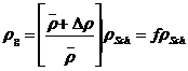
As shown in (Gonzalo & Alfonseca 2013) in more detail, equation (1) for an open universe with the KOFL model, k < 0, L = 0, can be solved analytically. The corresponding compact parametric solutions obtained are given by

,      ,                                 (2)

where , resulting in

,                         (3)

and

,                            (4)

Equation (3) is compatible with the observational evidence for the current value H₀t₀ = 0.9358 with this model, while the current relative density computed at equation (4) is W_m0 = W_m(y₀) = 0.0491 = W_b.

Taking into account that W_m evolves with time, that the density of the universe increases as we probe at higher distances, to evaluate the lensing effect we should consider, not the current density, but the variable density of the universe in the space traversed by light from its source to us. In the case of far protogalaxies, the furthest detected has (Wall 2012), not too far from the time when the universe stopped behaving as an exploding black hole (when it reached its Schwartzchild radius, R_Sch), just when  in this model. We can thus estimate the average density by averaging the values of W_m0 and W_mSch, which gives:

                                                      (5)

which results in = 5.59, close to the expected  relation in our neighbourhood (Weinberg 2008).

In this model, the dark matter effect on gravitational lensing could perhaps be explained, at least in part, because the average density of matter was much more dense at early times than it is at present. What our telescopes are seeing now is a superposition of snapshots of the universe since .

In the LCDM model (k = 0, L > 0), the density of the universe W=W_r+W_m+W_L relative to the critical density is assumed by hypothesis to be exactly equal to 1. The space-time curvature of the universe is assumed a priori to be flat, and therefore, there must be a lot of dark matter and a lot of dark energy to make (W_m + W_L) exactly equal to one (W_r being now negligible), where W_{m =} W_b + W_dm.

Equation (1) for a flat universe with the LCDM model can also be solved analytically. The corresponding compact parametric solutions obtained are

,                                                  (6)

where , resulting in

,                                               (7)

(H₀t₀ = 0.9476 with this model) and

,                            (8)

Curiously enough, equation (8) has the same shape as equation (4) for the KOFL model, although the meaning of the parameter y is different in both cases.

The derived current density is now W_m0 = 0.319. Computing the average density, as before, from the time when the universe reached its Schwarzchild radius and the present, we get:

,                                                        (9)

which  results in , much higher than the expected ratio of 6 (Weinberg 2008). This is something that requires a satisfactory explanation.

Figure 1a, which corresponds to Figure 9 in (Freedman et al 2001), with the horizontal axis modified to unify both models (KOFL and LCDM), shows clearly that both are compatible with the current estimations of H₀ and t₀. This is the same conclusion specified by (Freedman et al 2001). The same applies to a whole family of mixed cases, represented by the part of the horizontal dotted and dashed lines located between the vertical dotted and dashed lines. Figure 1b compares the evolution of W_m(y) with H(y)t(y): equation (4) vs equation (3) for the open universe (bottom curve), with 2/3<H(y)t(y)<1; equation (8) vs equation (7) for the flat universe (top curve), with 2/3<H(y)t(y)<¥. The current situation (H₀t₀) is represented in both models by the same abscissa (the dotted line), as the two values are almost indistinguishable at that scale. A horizontal line and separate arrows mark the half-density situation Ω_m(y)=1/2. The section tinted in light grey corresponds to the range of different solutions for the mixed cases (k<0 and L>0). The stronger parts of the two curves correspond to the density values we have averaged in the previous computation (between the time when the universe stopped behaving as an exploding black hole and the present situation). Notice that although both parts of Figure 1 seem to represent the same curves (exchanging the axes), the vertical axis of Figure 1a is not H(y)t(y) (as in the horizontal axis in Figure 1b), but H₀t₀ (different estimations for the current value of the product).

(a)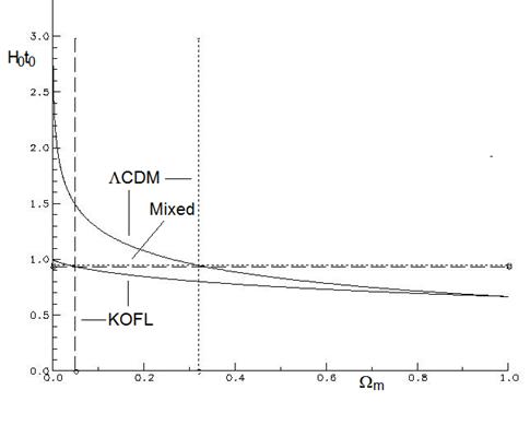

(b)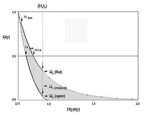

Figure 1. (a) Compatibility of the three models (KOFL, LCDM and mixed) with the current estimations of H₀ and t₀. Notice that H_ot_o>1 would invalidate the KOFL model. (b) Matter density parameter Ω_m(y) vs. dimensionless cosmic parameter H(y)t(y) = Hubble’s ratio ´ time for an open (KOFL), flat (ΛCDM) and mixed universe

One interesting difference between the models is the time when the universe would have reached its Schwarzchild radius, i.e. it stopped behaving like an exploding black hole. As indicated in Table 1, with the KOFL model this would have happened 414 million years after the Big Bang, at a redshift z=18.38, which means that the light of every object we have been able to detect was emitted by that object long after the universe could no longer be considered as a black hole. With the LCDM model, however, things are quite different, as the universe would have reached its Schwartzchild radius much later, over 3 billion years after the Big Bang, at a redshift z=2.134, which means that the light of some of the objects we have detected comes technically from within a black hole (see figure 2). This bizarre situation is difficult to explain.

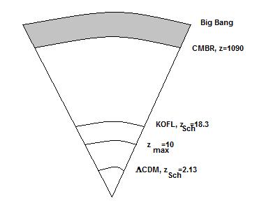
Figure 2. Relative situation of a few redshifts for an open (KOFL) and a flat (ΛCDM) universe

 

3.2. The CMB power spectrum

Another point of comparison between different models uses the situation at the time of Last Scattering (LS), about when the cosmic background microwave radiation was generated. As it is well known, the minute anisotropies in the CMB can be studied by means of spherical harmonics of order l = 0, 1, 2..., where the multipole moment l, detected by analyzing anisotropies at an angular separation qº, can be approximated by: l » 180º/qº. Theory states that l  < 100 represents anisotropies between points which at the time of last scattering were separated further than the horizon at that time (the distance where the expansion of the universe would have reached the speed of light), while l  > 100 represents anisotropies between points inside the horizon. The multipole corresponding to maximum anisotropy would take place, for different models, at about 200 for the LCDM model and at a higher value for the KOFL model (due to the high curvature assumed by this model (K=-1). Table II compares the results for both models.

Table 1I

Comparison of three different cosmological models: a flat (ΛCDM) universe with k=0, an open (KOFL) universe with Λ=0_, and a mixed universe with k=-0.5, Λ= Λ₀/2

 

Experimental measurements by the Planck satellite result in l _max » 200. It can be seen that the LCDM model fits better this result. The KOFL model, however, explains better the observations of high red-shift galaxies. The LCDM model can be adjusted in such a way that the multipole anisotropies for l  > 100 are predicted correctly, although the value obtained for H₀ (about 67) happens to be smaller than the value computed directly from Cepheid and supernovae observations in galaxies (about 73). This discrepancy should be explained (Friedman et al 2001, Siegfried 2014). On the other hand, the LCDM model is unable to explain the behavior of the multipole anisotropies for l  < 100. A mixed model with k<0 and Λ>0 has been offered as an alternative explanation (Aurich et al, 2004).

3.3. Questions about redshift

It is easy to check that the relativistic expression giving the distance r=R₀-R and velocity v, in terms of z (redshift),

                                                      (10)

                                                       (11)

result in

                                                           (12)

that for z << 1 results in the usual Hubble ratio

                ()

but for increasingly higher z values it gives

,                                                                          (13)

,                                                                         (14)

,                                                                            (15)

which mimics an accelerated expansion (a lower value in recession velocity at higher distances) completely unrelated to any non vanishing cosmological constant. Notice that we are neglecting the dipole component of our galaxy moving with respect to the CMBR at a speed of the order of c/1000.

When S. Perlmutter reported (Schwarzschild 2011) the accelerated expansion of distant type Ia supernovae, he pointed out that the apparent magnitudes reported might need corrections due to a possible dimming by interfering dust at early cosmic times. Let us make a quantitative evaluation of the corrections to the measured magnitudes due to dimming by cosmic dust. These corrections must be expected to bring down the observed magnitudes for high redshift type Ia supernovae, and to become negligible for supernovae closer to us, affected by much less cosmic dust (). Therefore they must become increasingly important for increasingly more distant supernovae (SN)(t_gf <t << t₀, with t_gf = galaxy formation time) beyond which no supernovae can be observed.

The uncorrected SN magnitude m^* and the correct one m would be given, respectively, by

,    ,

resulting in

                                                                                       (16)

in a direct relation to the light intensities (affected by the intervening dust) and  (unaffected), which are related to each other  by

                                                                                      (17)

where is the extinction coefficient, due to cosmic dust, which should be proportional to the cosmic density

Therefore

            (18)

that implies

                                                                     (19)

The correction in magnitude , which brings m in line with the distance vs. velocity relationship given by Eqs. (2), (3) is therefore:

,                                                                 (20)

which becomes  for small redshifts,  for z = 1 and  for z up to z_obs= (the currently maximum observed redshift).

The corrections are substantial even at moderate redshifts of the order of but the important point is that they may still be compatible with a small upwards curvature in the logarithmic magnitude versus velocity plots, therefore suggesting an accelerated expansion. This accelerated expansion would not have anything to do with a non- vanishing cosmological constant.

4. CONCLUDING REMARKS

The LCDM model has been considered standard in most publications on cosmology since 1998. However, the fitting of the Planck satellite experimental results to that model by (Ade et al 2013) cannot be considered a full validation, since there are still important discrepancies to be explained. It is interesting to notice that, when a detailed comparison was done in 2001 by Freedman and colleagues (Freedman et al 2001), their conclusion was: experimental data, at that time, were compatible with both the LCDM and KOFL models, as well as with a whole family of intermediate (mixed) models.

In this paper we have compared three different models, LCDM, KOFL for k=-1, and a mixed model, taking into account the values of H₀ and t₀ recently deduced from the data provided by Planck’s satellite. The first model implies the existence of large quantities of dark matter and dark energy, the second can be easily adjusted to predict none of them, the third occupies an intermediate position.

The KOFL model seems to have an important problem to solve: the behavior of the CMB anisotropies for multipoles l  > 100, especially the fact that it predicts a relatively high value for l_max. The LCDM model appears to be correct there, but still has several important problems to solve: a) a discrepancy between the inferred value of H₀ and the higher value obtained through astronomical observations; b) the behavior of the CMB anisotropies for multipoles l  < 100; c) the large quantities of dark matter and dark energy predicted, which nobody knows what they are and d) the fact that the light from the farthest objects currently detected (z»11) must have been emitted when the universe was technically still an exploding black hole. As to the current acceleration of the universe, as pointed out in section 3.3, it could also be fitted (at least in part) within a KOFL or a mixed model.

A more accurate determination of H₀ is clearly needed. Hopefully, NASA´s James Webb Space Telescope, to be launched in October 2018, will make it possible to compute it with an unprecedented precision,  less than 1% (private communication by John C. Mather, Principal Investigator).

Another point to be considered is the fact that the temperature of the universe at the time of last scattering is usually approximated to exactly 3000 K. Perhaps it should be noted that a slight change in this temperature (100 K up or down) moved the time when the CMBR happened by about 25,000 years in each direction.

The search for dark matter in WIMPS, axions and more exotic candidates has been going on for over three decades now. In spite of considerable experimental and theoretical efforts, it has been unsuccessful. Baryonic matter in early galaxies, whose light was emitted at times when the cosmic density was much higher than it is now, could account for at least some of the assumed effects of the elusive dark matter. On the other hand, at least a part of the cosmic acceleration currently attributed to dark energy could also be explained as a result of purely relativistic effects. Therefore, we should not assume that LCDM is the only alternative. Different models (such as the KOFL model or even mixed models) should be investigated and compared in depth, taking into account if their predictions of the maximum observable redshift from very distant early galaxies are compatible with astrophysical data.

 

Acknowledgements: We are very grateful to Professors Anthony Leggett and Francisco José Soler Gil,  as well as to Martín López Corredoira of the Astrophysical Institute in the Canary Islands, for reading carefully and critically our manuscript and for their encouragement to send it to a good journal in the field of Astrophysical Cosmology.

 

APPENDIX: ESTIMATION OF PROTOGALAXY FORMATION TIME

In this Appendix we show that the KOFL model requires a reasonable time for the first proto galaxies to be formed, so that the maximum observable red shifts may be expected to be substantially lower than z_Sch, the red shift corresponding to the universe´s Schwarzschild radius.

If we start from the KOFL model and assume that protogalaxies started forming by an aggregation of cosmic dust around a cosmic irregularity after the universe reached its Schwartzchild radius (when it stopped behaving like a black hole), their construction should have ended before the time of the maximum observed redshift (which currently is about 10), when galaxies can be observed now.

Let us estimate the protogalaxy formation time for a galaxy with mass M_g, so as to evaluate the order of magnitude of the maximum observable redshift. Variable r will represent the size of the galaxy during its formation, starting at zero (when the galaxy was just a cosmic irregularity) and ending at R_g when the galaxy was fully formed.

The protogalaxy radius R_g is related to the protogalaxy formation time by

                                                    (A21)

and the protogalaxy density is related to the cosmic average density and to the Schwarzschild density  (with M the mass of the universe) by

                                                               (A22)

where according to Peebles (quoted in Weinberg 2008, p. 424) the factor is of the order of 2.7.

The mean value of the bracketed factor in equation (13), for r in the interval can be evaluated by integrating it for that interval, giving

                                                                                                (A23)

Therefore, assuming that the galaxy had the same density as the universe at Schwarzschild time divided by :

                                                          (A24)

Using the data in Table 1 for the KOFL model and z_max»10 we get  and therefore , which implies

 Gyrs                              (A25)

resulting in Gyrs, therefore

                                                                     (A26)

quite close to the value 2.7 estimated by Peebles.

 

References

1. Ade, P.A.R. et al (261 authors) 2013, Planck 2013 results. XVI. Cosmological parameters, arXiv:1303.5076.
2. APS News 2013, 22, 6, p. 1.
3. Aurich, R., Lustig, S., Steiner, F., Then, H., Hyperbolic Universes with a Horned Topology and the CMB Anisotropy, Class.Quant.Grav. 21 (2004) 4901-4926. arXiv:0403597.
4. Einstein, Albert 1952, The Principle of Relativity (Toronto: Dover).
5. Freedman, Wendy L. et al (15 authors) 2001, Final Results from the Hubble Space Telescope to Measure the Hubble Constant. The Astrophysical Journal, 553:47-72.
6. Gonzalo, Julio A. 2012, Cosmic Paradoxes, chap. 6 (Singapore: World Scientific).
7. Gonzalo, Julio A. & Alfonseca, Manuel 2013, arXiv:1306.0238.
8. Jaki, Stanley L. 2000, The Paradox of Olbers Paradox (Pickney, MI: Real View Books).
9. Livio, M. & Riess, A.G. 2013, Measuring the Hubble constant, Physics Today 66, 10, 41.
10. Rees, Martin 2000, Just Six Numbers (New York: Basic Books).
11. Schwarzschild, B. M. 2011, Physics Today 64, 12, 14.
12. Siegfried, T. 2014, Cosmic Question Mark, Science News 185:7, 18-21, April 5, 2014.
13. Wall, Mike 2012, http://www.space.com/18879-hubble-most-distant-galaxy.html

14.  Weinberg, S. 2008, Cosmology (Oxford: Oxford University Press).